An Introduction to Qiskit and Quantum Computers

Introduction:

Quantum computers present a vastly different paradigm compared to traditional computers. Leveraging quantum bits (qubits) based on principles of quantum physics, quantum computers perform computations that offer potential to execute certain tasks much more efficiently than classical computers. Qiskit, an open-source quantum computing framework developed by IBM, is used to program and simulate quantum computers. In this article, we will provide an introduction to exploring quantum computers using Qiskit.

Learning Objectives:

1. Fundamental principles of quantum computers
2. Basic building blocks and usage of Qiskit
3. Creation and simulation of a simple quantum circuit
4. Analysis of simulation results

Introduction to Qiskit and Quantum Computers:

Qiskit is a Python-based library in the field of quantum computers and quantum computing. This library is used to create, simulate, and analyze quantum circuits. It provides developers with a powerful toolkit to understand the complexity of quantum computers and develop applications.

The fundamental building blocks of Qiskit are essential to understanding the principles of quantum computation. These building blocks include quantum bits (qubits), the basic components of quantum computers, and quantum gates used to manipulate them. Additionally, the simulation tools provided by Qiskit allow users to test and analyze quantum circuits, providing a platform to learn the fundamentals of quantum computing and explore the potential of quantum computers.

Code Review:

In this section of the article, we’ll provide a detailed review of the code that creates and simulates a simple quantum circuit using Python and the Qiskit library. We’ll explain how each step is performed and how the results are analyzed.

from qiskit import QuantumCircuit, Aer, transpile, assemble
from qiskit.visualization import plot_histogram

Here, we import necessary modules (QuantumCircuit, Aer, transpile, assemble, plot_histogram) from the Qiskit library. QuantumCircuit is used to create a quantum circuit, Aer provides the simulation backend, transpile and assemble functions prepare the circuit for simulation and send it to the processor, and plot_histogram is used for visualizing results.

class QuantumExample:
    def __init__(self):
        self.qc = QuantumCircuit(1, 1)  
        self.simulator = Aer.get_backend('qasm_simulator')
        self.compiled_circuit = None
        self.counts = None

We define a class named QuantumExample. In the constructor method (__init__), we define the attributes of the class: qc creates a quantum circuit, simulator defines a simulator backend, compiled_circuit and counts variables are used to store the circuit and results, respectively.

def build_circuit(self):
        self.qc.h(0)  
        self.qc.rz(0.3, 0)  
        self.qc.measure(0, 0)

The build_circuit method constructs the quantum circuit. The command qc.h(0) puts a qubit into superposition using a Hadamard gate. The command qc.rz(0.3, 0) rotates the qubit along the Z-axis by 0.3 radians. Finally, the command qc.measure(0, 0) measures the qubit.

def run_simulation(self):
        self.compiled_circuit = transpile(self.qc, self.simulator)
        job = assemble(self.compiled_circuit)
        result = self.simulator.run(job).result()
        self.counts = result.get_counts(self.qc)

The run_simulation method processes the created circuit and obtains simulation results. The transpile function prepares the circuit for simulation. The assemble function prepares the processed circuit as a job. The code simulator.run(job).result() executes the job and retrieves the result. Finally, the code result.get_counts(self.qc) retrieves the measurement results and saves them to the counts variable.

def visualize_results(self):
        print("Quantum Circuit:\n", self.qc)
        print("\nTranspiled Circuit:\n", self.compiled_circuit)
        print("\nMeasurement Results:", self.counts)
        plot_histogram(self.counts)

The visualize_results method visualizes the results. It first prints the quantum circuit and the transpiled circuit. Then, it prints the measurement results and visualizes them as a histogram.

if __name__ == "__main__":
    quantum_example = QuantumExample()
    quantum_example.build_circuit()
    quantum_example.run_simulation()
    quantum_example.visualize_results()

Finally, in the if __name__ == "__main__": block, an instance of the QuantumExample class is created, the quantum circuit is built, the simulation is run, and the results are visualized. This block enables the execution of the code.

Results and Analysis:

In this section, we will examine the simulation results of the quantum circuit and discuss the implications of the obtained results. Additionally, we will discuss how simulation results may differ on an improved quantum computer and potential applications.

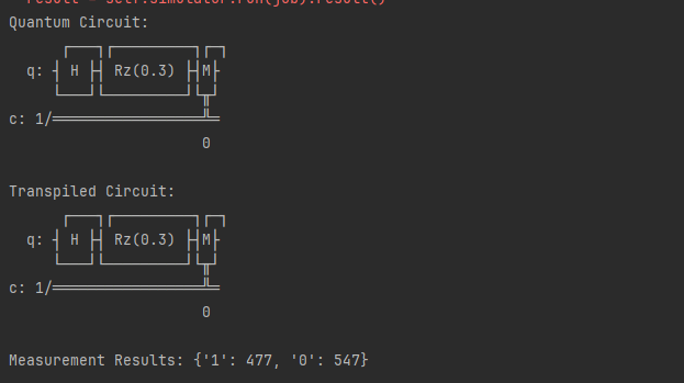
Quantum Circuit:

┌───┐┌─────────┐┌─┐
  q: ┤ H ├┤ Rz(0.3) ├┤M├
     └───┘└─────────┘└╥┘
c: 1/═════════════════╩═
                      0

In this part, the constructed quantum circuit is shown. The circuit includes a Hadamard gate (H) followed by a Z-axis rotation (Rz). The labels q and c represent quantum and classical bits, respectively. The operator M indicates the measurement of the qubit.

Transpiled Circuit:

┌───┐┌─────────┐┌─┐
  q: ┤ H ├┤ Rz(0.3) ├┤M├
     └───┘└─────────┘└╥┘
c: 1/═════════════════╩═
                      0

In this part, the processed version of the circuit is shown. The transpiled circuit is optimized and prepared for simulation. In fact, it is the same as the original since there is no need for optimization due to the simplicity of the circuit.

Measurement Results: {'1': 477, '0': 547}

The measurement results are the output of the simulation. These results provide the probabilities of ‘0’ or ‘1’ depending on the measurement outcome of the qubit. Here, it can be seen that there are 547 and 477 measurements with ‘0’ and ‘1’ values, respectively.

These results represent the statistical outcomes obtained when the simulation of the quantum circuit is run for a certain

period. Potentially, these results will be similar to those obtained on a real quantum computer, but they may differ when more complex circuits and more qubits are used.

Conclusion:

This article has provided a starting point for learning quantum computers using Qiskit. Understanding the basics of Qiskit’s usage will help readers take a step into the exciting world of quantum computing. After reading this article, readers will be encouraged to explore further advancements in the field of quantum computing.